Meshes with Python & Blender: Cubes and Matrices

Welcome to the sec­ond part in this series. It’s time to get into some math and learn how to con­trol the posi­tion, rota­tion and scale of the mesh.

This tuto­r­i­al builds on the lessons of part one. If you find your­self lost too often, try going back. Today we will quick­ly look into mak­ing cubes, and then jump into con­trol­ling the mesh and ori­gin point’s posi­tions. Finally we’ll dive into trans­for­ma­tion matri­ces and learn how to per­form trans­for­ma­tions nice and fast.

Tutorial Series

• Part 1: The 2D Grid
• Part 2: Cubes and Matrices
• Part 3: Icospheres
• Part 4: A Rounded Cube
• Part 5: Circles and Cylinders

The usual setup

Let’s start by import­ing the pack­ages we need. Besides the usu­al bpy, we are also going to use the radians() func­tion from Python’s math pack­age, as well as the Matrix class from mathutils (this one is from Blender).

import bpy
import math
from mathutils import Matrix

As before, I’ll have a sec­tion to put vari­ables in, then util­i­ty func­tions and final­ly the main code sec­tions. The vert() func­tion looks use­less now but we’ll need it for the next bit.

# -----------------------------------------------------------------------------
# Settings
name = 'Cubert'

# -----------------------------------------------------------------------------
# Utility Functions

def vert(x,y,z):
    """ Make a vertex """

    return (x, y, z)


# -----------------------------------------------------------------------------
# Cube Code

verts = []
faces = []


# -----------------------------------------------------------------------------
# Add Object to Scene

mesh = bpy.data.meshes.new(name)
mesh.from_pydata(verts, [], faces)

obj = bpy.data.objects.new(name, mesh)
bpy.context.scene.collection.objects.link(obj)

bpy.context.view_layer.objects.active = obj
obj.select = True

Making the cube

Making a cube is less glam­orous than you would expect since there’s no fan­cy algo­rithm to make them. Instead we have to input the vert posi­tions and faces man­u­al­ly. Luckily cubes only have 6 faces and 8 vertices.

verts = [vert(1.0, 1.0, -1.0),
         vert(1.0, -1.0, -1.0),
         vert(-1.0, -1.0, -1.0),
         vert(-1.0, 1.0, -1.0),
         vert(1.0, 1.0, 1.0),
         vert(1.0, -1.0, 1.0),
         vert(-1.0, -1.0, 1.0),
         vert(-1.0, 1.0, 1.0)]

faces = [(0, 1, 2, 3),
         (4, 7, 6, 5),
         (0, 4, 5, 1),
         (1, 5, 6, 2),
         (2, 6, 7, 3),
         (4, 0, 3, 7)]

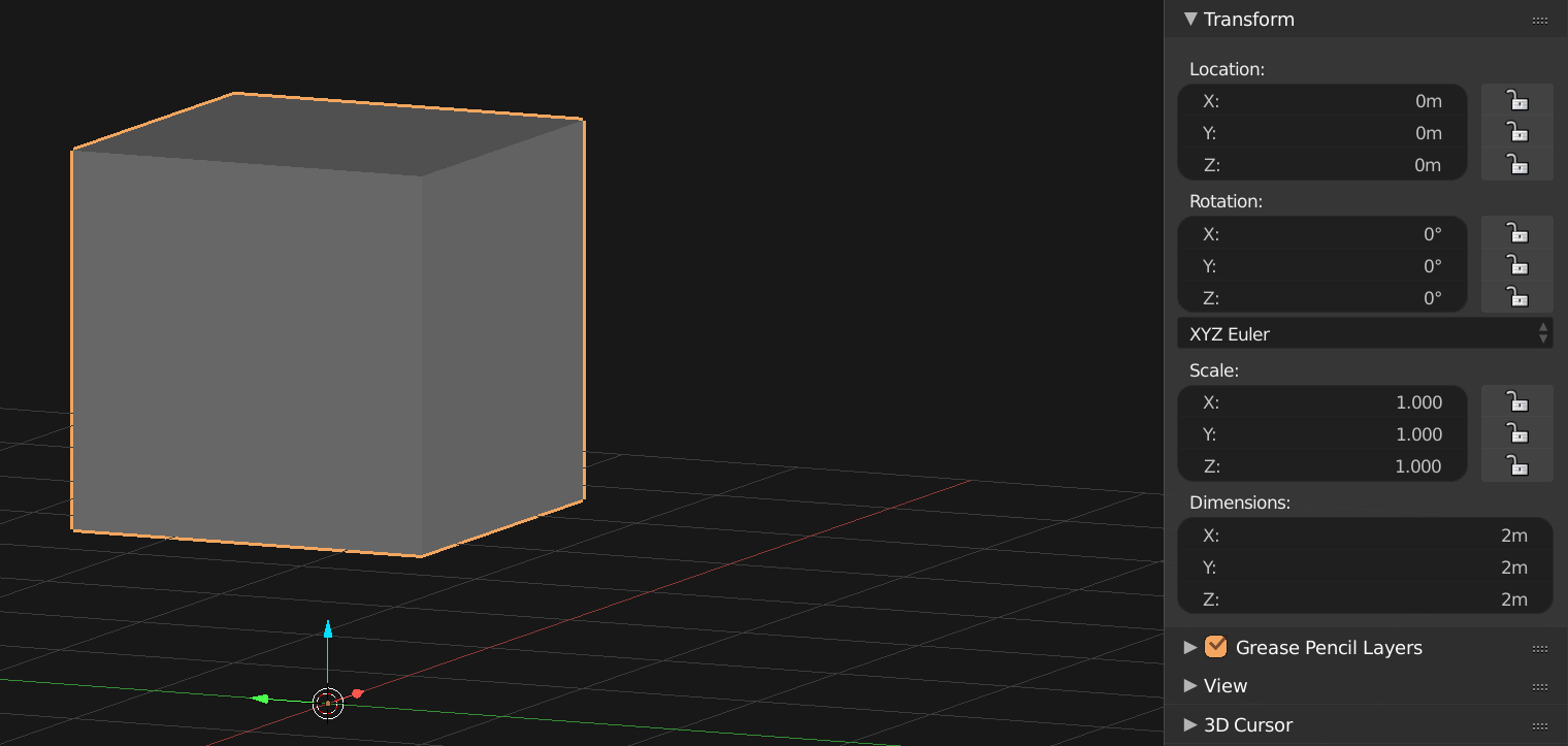
Run the script now and you will be reward­ed with a very default cube. Now that was easy! Let’s see what we can do with it.

Moving the origin point

Every object in Blender has an ori­gin point that deter­mines their posi­tion in 3D space. In fact when we talk about an object’s posi­tion we actu­al­ly talk about the posi­tion of its ori­gin point. On the oth­er hand when we talk about an ori­gin points’ posi­tion we actu­al­ly talk about the ori­gin points’ posi­tion rel­a­tive to the mesh.

Confused? Look at the fol­low­ing diagram.

As you can see when the orange dot (the ori­gin point) is on the grid, the object’s posi­tion is (0, 0, 0) while when it’s up by 1 on the Z axis the posi­tion is posi­tion is (0, 0, 1). But the inter­est­ing bit is the mesh’s posi­tion. In both cas­es the mesh is off­set by 1, but in the sec­ond case it is ‑1. If the mesh’s posi­tion was (0, 0, 0) it would be up in the air, right where the ori­gin is. As you can see, the mesh posi­tion is rel­a­tive to the ori­gin but inde­pen­dent from the origin’s posi­tion in the scene.

Knowing this, there are two things we can do:

• Change the mesh in rela­tion to the ori­gin point. This is the same as mov­ing the mesh in edit mode. 
• Change the ori­gin point while leav­ing the mesh in the same place. For this tuto­r­i­al that would be the cen­ter of the scene. 

We will begin by chang­ing the posi­tion of the mesh rel­a­tive to the ori­gin point I will be call­ing this off­set to keep things short.

offset = (0, 0, 1)

def vert(x,y,z):
    """ Make a vertex """

    return (x + offset[0], y + offset[1], z + offset[2])

We can use the vert func­tion to move the mesh with a sim­ple addition.

An off­set of 1 on Z will make the cube rest on the grid with the ori­gin point at its bottom.

Now let’s try mov­ing the ori­gin point while keep­ing the cube at the cen­ter of the scene. There’s only one small prob­lem: we can’t move the ori­gin itself. Moving the ori­gin is mov­ing the object, since the ori­gin rep­re­sents its posi­tion in space.

What we have to do is to change the ori­gin is move the mesh as before and move the object by the oppo­site of that offset.

obj.location = [i * -1 for i in offset]

Remember loca­tion is a tuple, so we have to use an expres­sion to set it.

Try run­ning the code now. The cube mesh is back at the cen­ter of the scene. But the ori­gin point (and the object) is now at (0, 0, ‑1).

Since we are chang­ing the loca­tion using the neg­a­tive of the off­set, the result­ing posi­tion of the object is neg­a­tive. Likewise using a neg­a­tive off­set results in a pos­i­tive posi­tion for the object. Give it a shot.

offset = (0, 0, -5)

So what if you want to change the ori­gin and also change the mesh posi­tion in any arbi­trary way so it’s not always at the cen­ter of scene? We can add anoth­er off­set to rep­re­sent that. And then we can add this off­set in the loca­tion expres­sion to move the mesh. Let’s also rename the pre­vi­ous off­set to keep things clear.

origin_offset = (0, 0, -5)
mesh_offset = (1, 0, 0)

def vert(x,y,z):
    """ Make a vertex """

    return (x + origin_offset[0], y + origin_offset[1], z + origin_offset[2])


obj.location = [(i * -1) + mesh_offset[j] for j, i in enumerate(origin_offset)]

Note that we have to use enumerate() now to get an index for the addition.

There are sev­er­al oth­er things we could do with expres­sions and the vert() func­tion. But there’s anoth­er way of trans­form­ing mesh­es and objects. A way that is both clean­er and faster.

Enter the Matrix

Matrices

In math matri­ces are rec­tan­gu­lar arrays of num­bers (and some­times oth­er things). They can be added, sub­tract­ed and mul­ti­plied between them­selves. You will find matri­ces in almost every field where math is involved.

The only field we care about though, is com­put­er graph­ics and in this con­text matri­ces are used often to rep­re­sent trans­for­ma­tions. This includes things like trans­la­tion, scal­ing or rota­tion. Matrices that rep­re­sent lin­ear trans­for­ma­tions like these are called “Transformation Matrices”.

Objects posi­tion, rota­tion and scale are defined as trans­for­ma­tion matri­ces in rela­tion to a coor­di­nate sys­tem. Even when you think there’s no transformation!

For instance, let’s imag­ine a “default object”. This object sits at coor­di­nates (0, 0, 0) of the scene, has a scale of 1 and a rota­tion of 0 (on all axis). We can rep­re­sent the loca­tion, scale or rota­tion of any object as a trans­for­ma­tion matrix of this default object. In Blender this is called a World Matrix, and it is a prop­er­ty avail­able in all objects.

By the way, “scene coor­di­nates” are actu­al­ly called “World Coordinates” in Blender. There are oth­er coor­di­nate spaces, as well as matri­ces for them but we will look into that in anoth­er part of this series (promise!).

Note that you don’t need to be a matrix wiz­ard to use them. The blender devs have blessed us with a Matrix class that does almost all the work for us, and you might not even have to see a matrix while you’re work­ing with them. Feel free to jump to “Putting it all togeth­er” if you’re not inter­est­ed in the math.

Still here? Alright, let’s play with this matrix con­cept for a moment. Go ahead and add a new object (using Shift+A). Select it, then paste this script on a text edi­tor and run it.

import bpy

print('-' * 80)
print('World Matrix \n', bpy.context.object.matrix_world)

You should see this out­put in the terminal:

--------------------------------------------------------------------------------
World Matrix
<Matrix 4x4 (1.0000, 0.0000, 0.0000, 0.0000)
            (0.0000, 1.0000, 0.0000, 0.0000)
            (0.0000, 0.0000, 1.0000, 0.0000)
            (0.0000, 0.0000, 0.0000, 1.0000)>

Since we haven’t moved, rotat­ed or done any­thing to the object, its val­ues are the same as our imag­i­nary “default object”. A matrix like this is called an Identity Matrix in math, and it means there’s no transformation.

Now move the cube some­where and run the script again.

--------------------------------------------------------------------------------
World Matrix
<Matrix 4x4 (1.0000, 0.0000, 0.0000, -8.8360)
            (0.0000, 1.0000, 0.0000, -1.1350)
            (0.0000, 0.0000, 1.0000,  8.9390)
            (0.0000, 0.0000, 0.0000,  1.0000)>

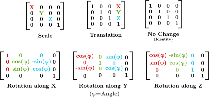
Aha! Now the matrix includes some change. The val­ues will be dif­fer­ent depend­ing on where you move the object. As you can see the last col­umn includes the X, Y, Z coor­di­nates in rela­tion to the cen­ter of the scene (world space).

What if we reset the loca­tion (Alt-G) and try scal­ing instead?

--------------------------------------------------------------------------------
World Matrix
<Matrix 4x4 (0.7280,  0.0000, 0.0000, 0.0000)
            (0.0000, -1.4031, 0.0000, 0.0000)
            (0.0000,  0.0000, 1.7441, 0.0000)
            (0.0000,  0.0000, 0.0000, 1.0000)>

Now the last col­umn has no change since the object is back at (0, 0, 0) However we can see three val­ues have changed to rep­re­sent scal­ing on X, Y and Z.

Rotation is more com­pli­cat­ed since you can rotate around three axis and each rota­tion is rep­re­sent­ed by trans­for­ma­tions on the oth­er two axis. This goes a bit out of scope for this tuto­r­i­al, so I’ll leave sev­er­al links at the end in case you want to get deep­er into the math.

--------------------------------------------------------------------------------
World Matrix
<Matrix 4x4 (-0.9182,  0.3398, -0.2037, 0.0000)
            (-0.2168, -0.8612, -0.4597, 0.0000)
            (-0.3316, -0.3780,  0.8644, 0.0000)
            ( 0.0000,  0.0000,  0.0000, 1.0000)>

You might also be won­der­ing about the last row. Transformation matri­ces for 3D are actu­al­ly 4D, the last row is an extra dimen­sion. This is a math­e­mat­i­cal “trick” to enable the matrix to per­form trans­la­tions. Again, I won’t get too tech­ni­cal about this. Check the links at the end for more info. In any case, it’s not impor­tant for our pur­pos­es since it will nev­er change.

Here’s a dia­gram of the dif­fer­ent transformations:

Using Matrices

Transformation matri­ces can be com­bined to cre­ate a sin­gle matrix that includes all the result of all the trans­for­ma­tions. This is done by mul­ti­ply­ing them. That means we can take an object’s world matrix and mul­ti­ply it by a trans­for­ma­tion matrix to get a new matrix that includes the changes in both matri­ces. We can then assign it as the object’s world matrix and thus trans­form the object.

Or to put it in code:

obj.matrix_world @= some_transformation_matrix

It’s time to whip out that Matrix class and see how we can use it to gen­er­ate matrices.

Translation

Let’s start with the eas­i­est: mov­ing stuff. All we have to do is call the Translation method of the Matrix class with a vec­tor (or tuple) of val­ues for each axis.

translation_matrix = Matrix.Translation((0, 0, 2))
obj.matrix_world @= translation_matrix

Scaling

Scaling takes three argu­ments. The first one is the scale fac­tor. The sec­ond one is the size of the matrix, it can be either 2 (2×2) or 4(4x4). But since we are work­ing with 3D objects this should always be 4. The final argu­ments is a vec­tor to spec­i­fies the axis to scale. This can be either zero for no scal­ing, or 1 to scale.

scale_matrix = Matrix.Scale(2, 4, (0, 0, 1)) # Scale by 2 on Z
obj.matrix_world @= scale_matrix

Rotation

Rotation takes almost the same argu­ments as scale. The first is the angle of rota­tion in radi­ans. The sec­ond is the size of the matrix (same as before). And the third is the axis of the rota­tion. You can pass a string like ‘X’, ‘Y’ or ‘Z’, or a vec­tor like the one in scale.

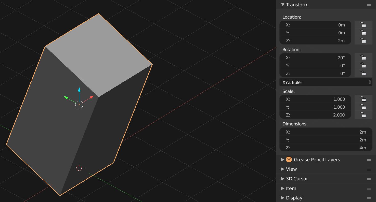
rotation_mat = Matrix.Rotation(math.radians(20), 4, 'X')
obj.matrix_world @= rotation_mat

Putting it all together

We can chain trans­for­ma­tions togeth­er by mul­ti­ply­ing them one after the oth­er. But beware, Matrix mul­ti­pli­ca­tion is not com­mu­ta­tive. Order does mat­ter. Start by trans­la­tion, then rota­tion and scale. If you’re get­ting strange val­ues that look like round­ing errors, look at the order in which you are multiplying.

translation = (0, 0, 2)
scale_factor = 2
scale_axis = (0, 0, 1)
rotation_angle = math.radians(20)
rotation_axis = 'X'

translation_matrix = Matrix.Translation(translation)
scale_matrix = Matrix.Scale(scale_factor, 4, scale_axis)
rotation_mat = Matrix.Rotation(rotation_angle, 4, rotation_axis)

obj.matrix_world @= translation_matrix @ rotation_mat @ scale_matrix

Matrices can also be used to change the mesh instead of the object. To do this we can use the transform() method of in objects. All it asks for is that you give it a matrix.

obj.data.transform(Matrix.Translation(translation))

Don’t for­get we can also com­bine matri­ces by mul­ti­pli­ca­tion so you can do sev­er­al trans­for­ma­tions in one go.

obj.data.transform(translation_matrix @ scale_matrix)

Not only are matri­ces faster but this method also goes straight to C, so it per­forms con­sid­er­ably bet­ter than cal­cu­lat­ing the posi­tion of each ver­tex in Python (which is quite slow and expen­sive). On top of that, we can do this in a sin­gle line.

Awesome.

Final code

import bpy
import math
from mathutils import Matrix

# -----------------------------------------------------------------------------
# Settings

name = 'Cubert'

# Origin point transformation settings
mesh_offset = (0, 0, 0)
origin_offset = (0, 0, 0)

# Matrices settings
translation = (0, 0, 0)
scale_factor = 1
scale_axis = (1, 1, 1)
rotation_angle = math.radians(0)
rotation_axis = 'X'


# -----------------------------------------------------------------------------
# Utility Functions

def vert(x,y,z):
    """ Make a vertex """

    return (x + origin_offset[0], y + origin_offset[1], z + origin_offset[2])


# -----------------------------------------------------------------------------
# Cube Code

verts = [vert(1.0, 1.0, -1.0),
         vert(1.0, -1.0, -1.0),
         vert(-1.0, -1.0, -1.0),
         vert(-1.0, 1.0, -1.0),
         vert(1.0, 1.0, 1.0),
         vert(1.0, -1.0, 1.0),
         vert(-1.0, -1.0, 1.0),
         vert(-1.0, 1.0, 1.0)]


faces = [(0, 1, 2, 3),
         (4, 7, 6, 5),
         (0, 4, 5, 1),
         (1, 5, 6, 2),
         (2, 6, 7, 3),
         (4, 0, 3, 7)]


# -----------------------------------------------------------------------------
# Add Object to Scene

mesh = bpy.data.meshes.new(name)
mesh.from_pydata(verts, [], faces)

obj = bpy.data.objects.new(name, mesh)
bpy.context.scene.collection.objects.link(obj)

bpy.context.view_layer.objects.active = obj
obj.select = True

# -----------------------------------------------------------------------------
# Offset mesh to move origin point

obj.location = [(i * -1) + mesh_offset[j] for j, i in enumerate(origin_offset)]


# -----------------------------------------------------------------------------
# Matrix Magic

translation_matrix = Matrix.Translation(translation)
scale_matrix = Matrix.Scale(scale_factor, 4, scale_axis)
rotation_mat = Matrix.Rotation(rotation_angle, 4, rotation_axis)

obj.matrix_world @= translation_matrix @ rotation_mat @ scale_matrix


# -----------------------------------------------------------------------------
# Matrix Magic (in the mesh)

# Uncomment this to change the mesh
# obj.data.transform(translation_matrix @ scale_matrix)

Wrap up

This cov­ers this part in the series. If Matrices have peaked your inter­est here’s a few links to learn more. The links are in order of difficulty.

• World Matrix Documentation on Blender’s API
• Computerphile’s video on Matrices
• Matrices (Wikipedia)
• Transformation Matrices (Wikipedia)
• Matrix Multiplication (Wikipedia)
• Scratchapixel’s les­son on matrices
• Coding Labs’article on Projection Transformation Matrices

A few things you can try to do yourself:

• Put this all in a loop and make mul­ti­ple cubes fol­low­ing a sequen­cial trans­for­ma­tion, like mak­ing a wave or rotat­ing around an axis.
• Use matri­ces to move the ori­gin of the cube, using the method in this tutorial
• Try scal­ing the mesh with­out matri­ces or chang­ing the object’s coor­di­nates (hint: don’t for­get the vert() function)
• Try apply­ing the world matrix of one object into another

In the next tuto­r­i­al we’ll be look­ing at mak­ing Icosahedrons and sub­di­vid­ing them to approx­i­mate a sphere. Do you have any ques­tions, or sug­ges­tions for the next tuto­ri­als? Leave a com­ment below!